on
Final Election Prediction
#Updated Model When predicting the 2022 midterm elections, I decided to create a linear regression model based on variables from 3 categories: 1) expert predictions, 2) economic indicators, and 3) demographic variables. Included in expert predictions are three variables that are coded as dummy variables: whether it is a close election or not, whether voters are Lean, Likely, or Safe Democrats, and whether or not the President is a Democrat or not. I also used 2 economic indicators of U.S. CPI (Consumer Price Index) and Unemployment Rate. The demographic variables included the characteristics of voters who were female, age 20-29, or White.
##
## Call:
## lm(formula = DemVotesMajorPercent ~ Close_E_D + LLS_D + Pres_D +
##     US_CPI + US_UEP_Rate + female + X20_29 + white, data = final_data_1106)
##
## Residuals:
##     Min      1Q  Median      3Q     Max
## -15.623  -2.110   0.113   1.862  19.192
##
## Coefficients:
##             Estimate Std. Error t value Pr(>|t|)
## (Intercept) 27.32918   10.97670   2.490  0.01312 *
## Close_E_D   11.89708    0.42671  27.881  < 2e-16 ***
## LLS_D        5.69332    0.38756  14.690  < 2e-16 ***
## Pres_D      -2.55847    0.88091  -2.904  0.00385 **
## US_CPI      -0.06183    0.01571  -3.935 9.56e-05 ***
## US_UEP_Rate  0.26367    0.23542   1.120  0.26328
## female      57.40102   18.55901   3.093  0.00210 **
## X20_29      19.91099    7.17390   2.775  0.00573 **
## white       -2.43858    1.01222  -2.409  0.01637 *
## ---
## Signif. codes:  0 '***' 0.001 '**' 0.01 '*' 0.05 '.' 0.1 ' ' 1
##
## Residual standard error: 3.608 on 479 degrees of freedom
## Multiple R-squared:  0.656,  Adjusted R-squared:  0.6503
## F-statistic: 114.2 on 8 and 479 DF,  p-value: < 2.2e-16
#(1) Prediction Model Formula
Y = 27.32918 + 11.89708X1 + 5.69332X2 - 2.55847X3 - 0.06183X4 + 0.26367X5 + 57.40102X6 + 19.91099X7 – 2.43858X8
whereas, Y = Democratic Party Popular Vote Share of two major parties (in %) [100-Y = Republican Popular Vote Share of two major parties (in %)]
          X1 = Dummy for Close (Toss-up) Election
                  if votes for either candidate < 60% (i.e., margin < 20%), 1
                  otherwise, 0

          X2 = Dummy for Lean, Likely, or Solid for Democratic candidate
                  if votes for Democratic candidate > 60%, 1
                otherwise, 0

        X3 = Dummy for Democratic President
                if President is Democrat, 1
                otherwise, 0

        X4 = US Consumer Price Index (consumer price level of 1982-84 = 100)

        X5 = US Unemployment Rate (annual average, in %)

          X6 = Share of Female Population among Total Voting Age Population

          X7 = Share of Population (aged 20-29) among Total Voting Age Population

          X8 = Share of White Non-Hispanic Single Race Population among Total
            Voting Age Population
The actual prediction of national popular vote share for the two parties (Democrat and GOP) in the 2022 House of Representatives election is summarized in section (5).
#(2) Model Description and Justification
The specified prediction model in section (1) is a multivariate regression model that estimates the popular vote share of Democratic Party for House Representative elections using the past five House Representative election results from 2012 to 2020. The unit of observation is congressional districts in the U.S. Not all the variables are available for the 2012-2022 study period, so the total number of sample observations used to specify the multivariate regression model is 488. This is mainly due to the availability of raw data about expert rating from “FiveThirtyEight.”
The dependent variable is the Democratic Party vote share out of the total votes to two parities (Democratic and Republican). The proposed model has three groups of independent variables: (i) Political Environment captured by how competitive election is and who is in White House; (ii) Macroeconomic Performance in the U.S. represented by Consumer Price Level, and Labor Market situation (unemployment rate); (iii) Demographic Characteristics of Voting Age Population represented by shares of female, young voters in 20s, and white non-Hispanic voters. The coefficients for all variables except for unemployment rate variable show the expected signs and significant at 5% level. (Details are explained in the following sections.) It is important to consider how close the election is when estimating the popular vote share since this can increase the voter turnout rate. Also, President’s party historically tends to have disadvantages in House elections. National macroeconomic performance can serve as critical factors for voters as well. Demographic characteristics of voters are important to predict the election results, e.g., in an election where majority of voters are more progressive such as younger voters, female, and minority in race, Democratic party’s popular votes tend to increase.
According to the FiveThirtyEight prediction of national popular vote for 2022 House Representative election, popular vote margin is in favor of Republican party, ranging from 2.3% on Sep 23, 2022 to 6.6% on June 13. In other words, the margin has never been greater than 20%, indicating that 2022 House Representative election is Toss-up election when measured by popular vote. That is why the value of dummy variables (X1 is set to be one, while X2 is set to be zero).
#(3) Coefficients of Multivariate Regression Model
All the coefficients in the proposed multivariate regression model are significant at 5% level as shown below.
Variable Coefficient Estimate Std. Error t-value Prob. (>|t|)
(Intercept) 27.32918 10.9767 2.49 0.01312 X1 (Close_E_D) 11.89708 0.42671 27.881 < 2.00E-16 X2 (LLS_D) 5.69332 0.38756 14.69 < 2.00E-16 X3 (Pres_D) -2.55847 0.88091 -2.904 0.00385 X4 (US_CPI) -0.06183 0.01571 -3.935 9.56E-05
X5 (US_UEP_Rate) 0.26367 0.23542 1.12 0.26328
X6 (female) 57.40102 18.55901 3.093 0.0021 X7 (X20_29) 19.91099 7.1739 2.775 0.00573
X8 (white) -2.43858 1.01222 -2.409 0.01637 *
Signif. codes: 0 ‘***’ 0.001 ‘**’ 0.01 ‘*’ 0.05 ‘.’ 0.1 ‘ ’ 1**For additional estimation results including residuals, R-squared values, and F-statistics, see below.
lm (formula = DemVotesMajorPercent ~ Close_E_D + LLS_D + Pres_D + US_CPI + US_UEP_Rate + female + X20_29 + white, data = final_data_1106)
Residuals: Min 1Q Median 3Q Max -15.623 -2.110 0.113 1.862 19.192
Residual standard error: 3.608 on 479 degrees of freedom (45 observations deleted due to missingness) Multiple R-squared: 0.656, Adjusted R-squared: 0.6503 F-statistic: 114.2 on 8 and 479 DF, p-value: < 2.2e-16
#(4) Interpretation of Coefficients
An estimated coefficient of the model is the marginal effect of an independent variable on the dependent variable (Democratic Party Votes Share out of Total Votes to Democratic and Republican parties). Individual marginal effects of all independent variables are summarized below.
X1 (Close_E_D): varies by district and election year If FiveThirtyEight prediction shows that an election is toss-up (i.e., votes for either candidate < 60%, or margin between the candidates of two parties < 20%) in a congressional district, Democratic vote share increases by 11.89708 % compared to the non-toss-up cases.
X2 (LLS_D): varies by district and election year If FiveThirtyEight prediction shows that an election is lean, likely, or solid for a Democratic candidate (i.e., Democratic candidate > 60%) in a congressional district, Democratic vote share increases by 5.69332 % compared to the other cases including toss-up and lean, likely, or solid for a Republican candidate.
X3 (Pres_D): varies by election year If the current president is from Democratic party, Democratic vote share decreases by 2.55847 % compared to the elections with a president from non-Democratic party (Republican party or any other parties).
X4 (US_CPI): varies by election year With one point increase in Consumer Prices Index in the U.S. (CPI in 1982-84 is at 100) from BLS (Bureau of Labor Statistics), Democratic vote share decreases by 0.06183%.
X5 (US_UEP_Rate): varies by election year Since the coefficient is not significant at 5% level, the national unemployment rate (=unemployed/total labor force) from BLS (Bureau of Labor Statistics) does not have statistically meaningful marginal effect on Democratic vote share increases.
X6 (female): varies by district and election year With one percent increase in the share of female population out of total voting age population in a congressional district (raw data from ACS of US Census), Democratic vote share increases by 0.5740102%.
X7 (X20_29): varies by district and election year With one percent increase in the share of population aged from 20 to 29 out of total voting age population in a congressional district (raw data from ACS of US Census), Democratic vote share increases by 0.1991099%.
X8 (white): varies by district and election year With one percent increase in the share of Single Race White Non-Hispanic population out of total voting age population in a congressional district (raw data from ACS of US Census), Democratic vote share decreases by 0.0243858%.
The coefficients of the model can be utilized to predict the nationwide Democratic vote share when the U.S. average values of the independent variables (that vary by congressional districts) are used. For instance, the U.S. average values of the eight independent variables can be calculated from the raw data for 2022 or the most up-to-date information and inputted to predict the nationwide Democratic vote share for the 2022 House Representative Election.
##        1
## 50.55775
## 1
## 50.46881#(5) Prediction & Model Validation
Prediction Results for 2022 House Election: To make a prediction of nationwide Democratic Party Vote Share of the two major party votes, the proposed multivariate regression model is used. For the 2022 House Representative Election, the most recent data available are used at national level from various data sources. Details are summarized in the table below.
The predicted nationwide Democratic Party vote share of 2022 House Representative Election is 50.56%, whereas the matching share for Republican Party is 49.44% (=100% -50.56%). Consequently, the margin between two major parties is expected to be 1.12%.
Variable Coefficient Estimate U.S. Avg. for 2022 Data Source (C) (A) (B) (Year) = (A) * (B) (Intercept) 27.32918 N/A N/A 27.32918 X1 (Close_E_D) 11.89708 1 FiveThirtyEight (2022) 11.89708 X2 (LLS_D) 5.69332 0 FiveThirtyEight (2022) 0 X3 (Pres_D) -2.55847 1 White House (2022) -2.55847 X4 (US_CPI) -0.06183 296.80800 US BLS (2022) -18.35164 X5 (US_UEP_Rate) 0.26367 3.79194 US BLS (2022) 0.99982 X6 (female) 57.40102 0.50975 ACS (2021) **** 29.26017 X7 (X20_29) 19.91099 0.17423 ACS (2021) **** 3.46909 X8 (white) -2.43858 0.60972 ACS (2021) **** -1.48685
SUM of Column (C) (National Democratic Vote Share of 2022 House Representative Election 50.55775 (=50.56%)
- This is an intercept shown in column (A) and it is not multiplied with the value in column (B). ** US BLS (Bureau of Labor Statistics) – CPI data for September 2022 *** US BLS – Annualized Unemployment Rate for 2021 & 2022 **** ACS (American Community Survey) of US Census – 2021 ACS 1% Sample Data
Additionally, the prediction for the most competitive district in Nevada (NV-3) was made using the proposed model. The demographic characteristics of the district (NV-3) from ACS 2021 data and U.S. macroeconomic conditions with the expert ratings for the election are used to estimate the popular vote share of the Democratic candidate in District 3. The predicted Democratic candidate (Susie Lee) vote share in NV-3 for the 2022 House Representative Election is 50.47%, whereas the matching share for Republican candidate (Dan Rodimer) is 49.53% (=100% -50.47%). Consequently, the margin between two major parties is expected to be 0.94%.
## [1] 0.6559999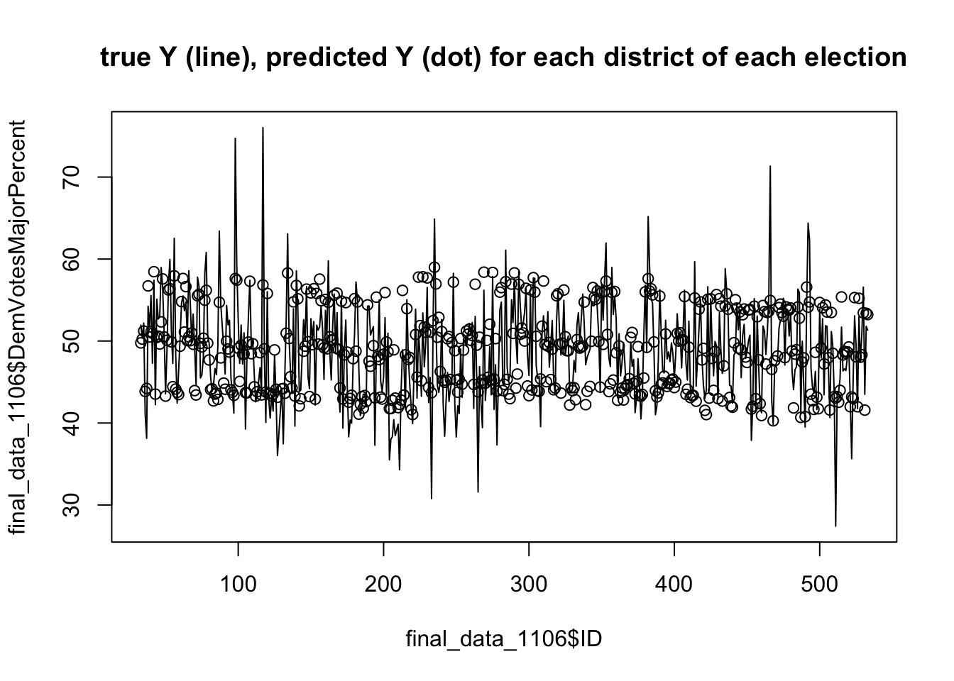
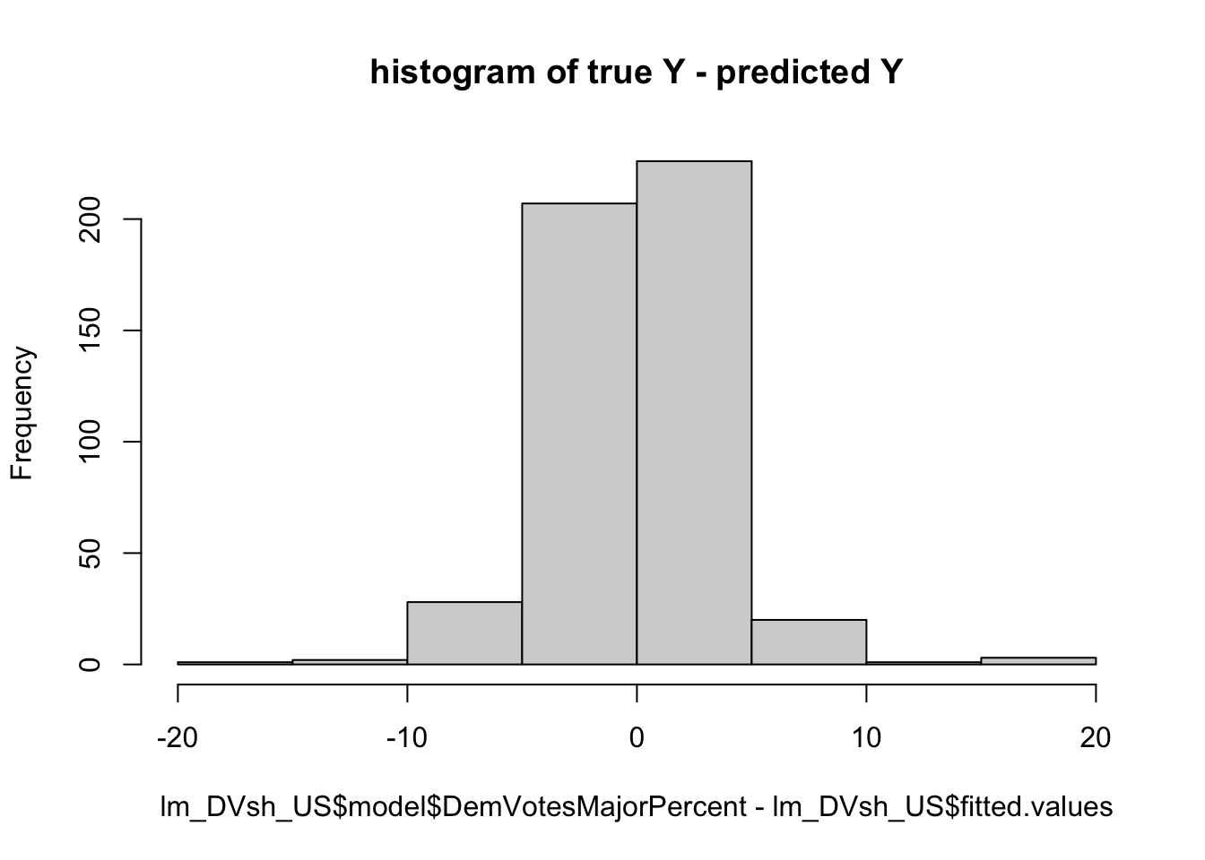
## [1] 3.574183In-sample Model Validation: With the aim to evaluate the predictive power of the model, I checked the in-sample fit. The first measure is R-square of the model. The R-square value of the prediction model is 0.6559999, indicating that the 65.60% of the total variation in the Y, the dependent variable (Democratic Party vote share) is explained by the proposed multivariate regression model, while the rest (34.40%) is due to errors (not captured by the proposed regression model).
Additionally, in-sample error can be displayed in the two graphs above. The first graph plots the in-sample error via residuals, which capture the difference between each observed (true) value of Y (in line) and predicted value of Y (in dots). The second graph plots the in-sample error via residuals in histogram, which visualizes the frequency of the difference between each observed (true) value of Y and predicted value of Y. Finally, RMSE (Square Root of Mean Squared Error) can be used to quantify how well a model fits a dataset with a single number. The calculated RMSE of the model is 3.574183 that shows the average distance between the observed values and the predicted values of Democrat Vote Share (the dependent variable).
##
## Call:
## lm(formula = DemVotesMajorPercent ~ Close_E_D + LLS_D + Pres_D +
##     US_CPI + US_UEP_Rate + female + X20_29 + white, data = final_data_1106[final_data_1106$year !=
##     2018, ])
##
## Residuals:
##      Min       1Q   Median       3Q      Max
## -14.6174  -2.1125   0.0213   1.8406  17.7046
##
## Coefficients:
##             Estimate Std. Error t value Pr(>|t|)
## (Intercept) 36.28772   12.14205   2.989  0.00300 **
## Close_E_D   12.74247    0.49956  25.508  < 2e-16 ***
## LLS_D        6.45968    0.44922  14.380  < 2e-16 ***
## Pres_D      -2.29460    0.86242  -2.661  0.00816 **
## US_CPI      -0.11869    0.01658  -7.160 4.91e-12 ***
## US_UEP_Rate  1.33113    0.25864   5.147 4.47e-07 ***
## female      49.13679   20.79129   2.363  0.01867 *
## X20_29      20.24902    8.10917   2.497  0.01299 *
## white       -2.25886    1.16986  -1.931  0.05432 .
## ---
## Signif. codes:  0 '***' 0.001 '**' 0.01 '*' 0.05 '.' 0.1 ' ' 1
##
## Residual standard error: 3.525 on 344 degrees of freedom
## Multiple R-squared:  0.7061, Adjusted R-squared:  0.6993
## F-statistic: 103.3 on 8 and 344 DF,  p-value: < 2.2e-16
## [1] 0.706106## [1] 6.621018## [1] 0.3898562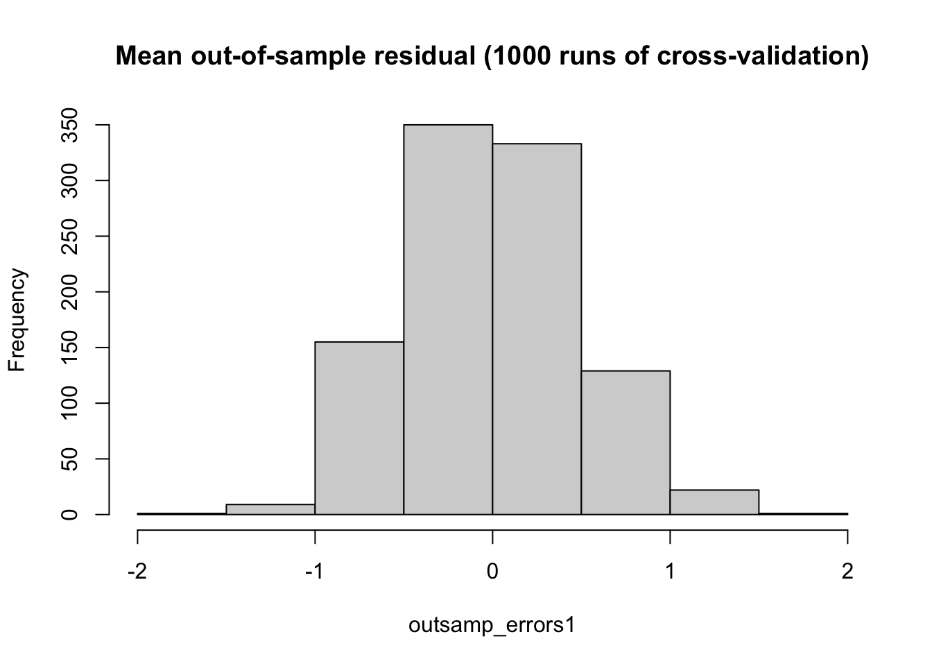 Out-of-sample Model Validation:
Another way to evaluate the predictive power of the model is to simulate out-of-sample prediction by withholding some observations before fitting. With a smaller sample by dropping 2018 observations from the dataset, I can estimate a new (modified) prediction model which will be used to predict the Y2018 (Democrat Vote Share in 2018 election). The newly modified model (lm_DVsh_US_no_2018) has the same set of independent variables but with different coefficients. Also, the R-square of this newly modified model is different from the original model with all observations including the sample from 2018 election. The R-squared value of the modified model is 0.7061. In the next steps, I predicted the values of the Y2018 (Democrat Vote Share in 2018 election) and compared the 135 predicted values with the true (observed) values of the 2018 election. The difference between each observed (true) value of Y2018 and predicted value of Y2018 is the difference between each observed (true) value of Y and predicted value of Y, using the out-of-sample prediction model. From the differences, I can see how well the modified model predicts the (true) value of Y2018 for the held-out observations X2018. RMSE of the out-of-sample model is 6.621018, higher than the all sample RMSE of 3.574183. This reveals that out-of-sample model works significantly worse than the in-sample model with all dataset. With a “Cross-validation.” I repeatedly evaluating performance against many randomly held-out “out-of-sample” datasets, for 1,000 times by dropping randomly selected 100 samples. The graph (Mean out-of-sample residual) above shows the distribution of evaluations in a histogram. The mean of the absolute value of errors from the 1,000 simulations is 0.3972904.
##        fit      lwr      upr
## 1 50.55775 43.01576 58.09973
## fit lwr upr
## 1 50.46881 42.91322 58.0244#(6) Uncertainty around Prediction (Predictive Interval)
As shown above for 2018 election case, the 95% predictive interval ranges from 49.04% to 63.31%, which includes the predicted national Democrat Vote Share in 2018 House Representative election (56.17%), 1.82% higher than the actual national vote share of Democratic Party in 2018 House Representative election.
The proposed multivariate regression model predicted the national Democrat Vote Share in 2022 House Representative election, which is 50.56 Representative Election has its fit value of 50.55775% with the 95% of prediction interval ranging from 43.01576% (lower bound) to 58.09973% (upper bound). It means that the 2022 national Democratic vote share of House Representative election would fall in this prediction interval with 95% of probability.
fit lwr uprU.S. 50.55775 43.01576 58.09973
Again, all the estimation (prediction) model comes with a certain level of errors which translates into uncertainty of the model. That is why it is important to check the interval of a prediction.
The prediction interval for NV-3 district is also estimated. The Democratic candidate (Susie Lee) is expected to win with an estimated vote share of 50.47% against the Republican candidate (Dan Rodimer). With 95% of prediction interval, the lower bound of the popular vote share of Democratic candidate is 42.91% and the upper bound is 58.02%.
fit lwr uprNV-3 50.46881 42.91322 58.0244
#(7) Graphs showing prediction
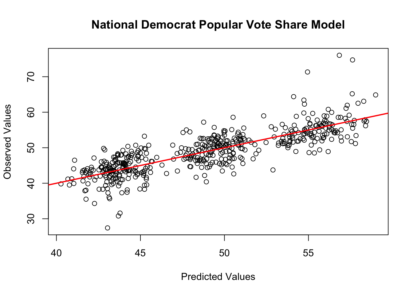
National Democrat Vote Share Graph: The first graph shows the scatter plot of the predicted values of the regression model on the horizontal-axis and the observed values of the model on the vertical axis. The red line is the best-fitted line of the scatter plot. If the model perfectly predicted with R-squared value of 1, all the points would have been on the best-fitted line with a slope of 1.
## `geom_smooth()` using formula 'y ~ x'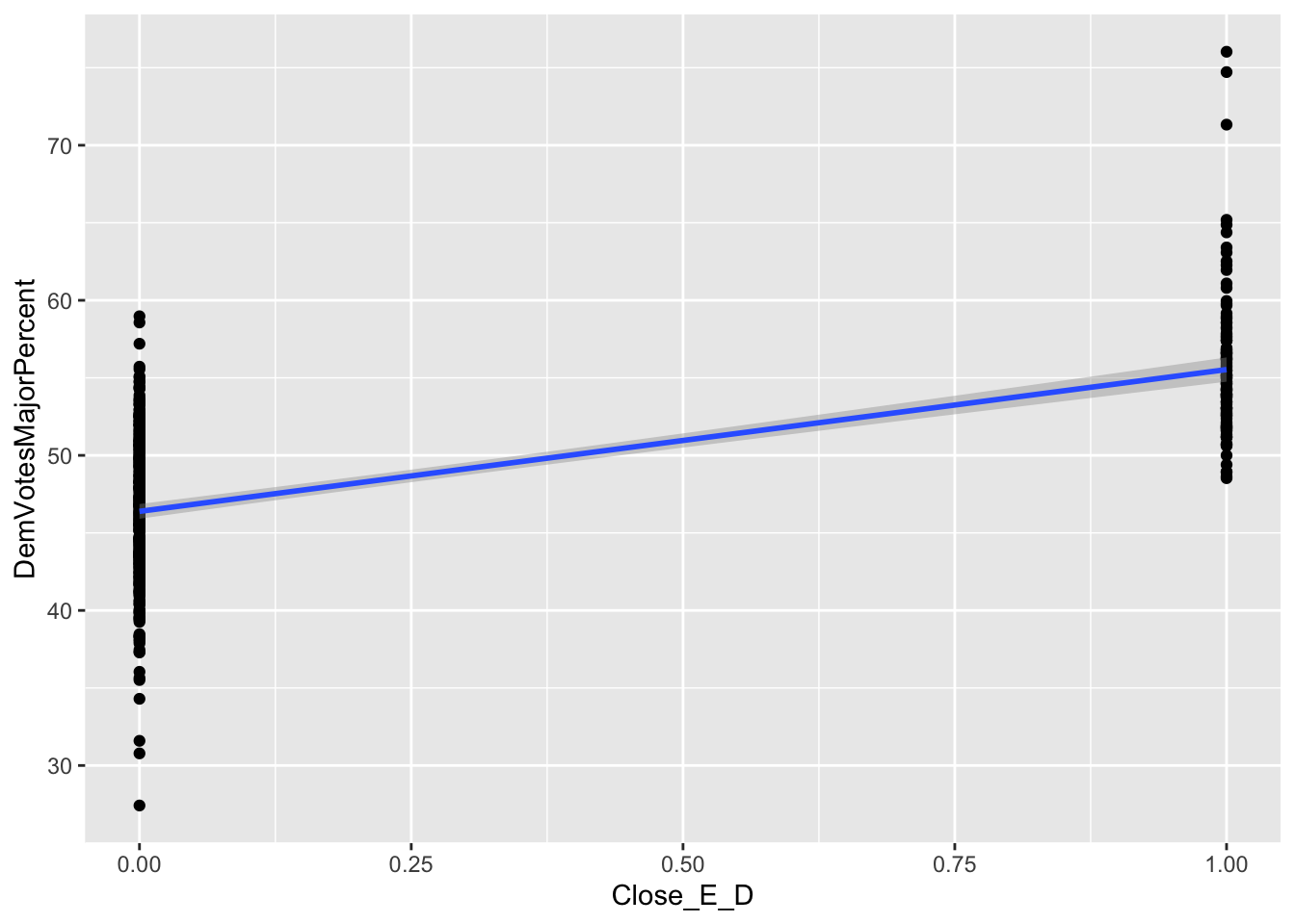
## `geom_smooth()` using formula 'y ~ x'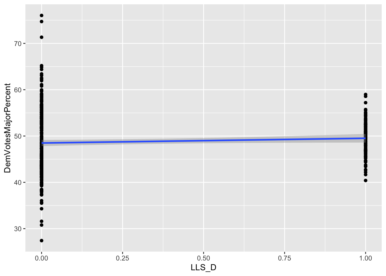
## `geom_smooth()` using formula 'y ~ x'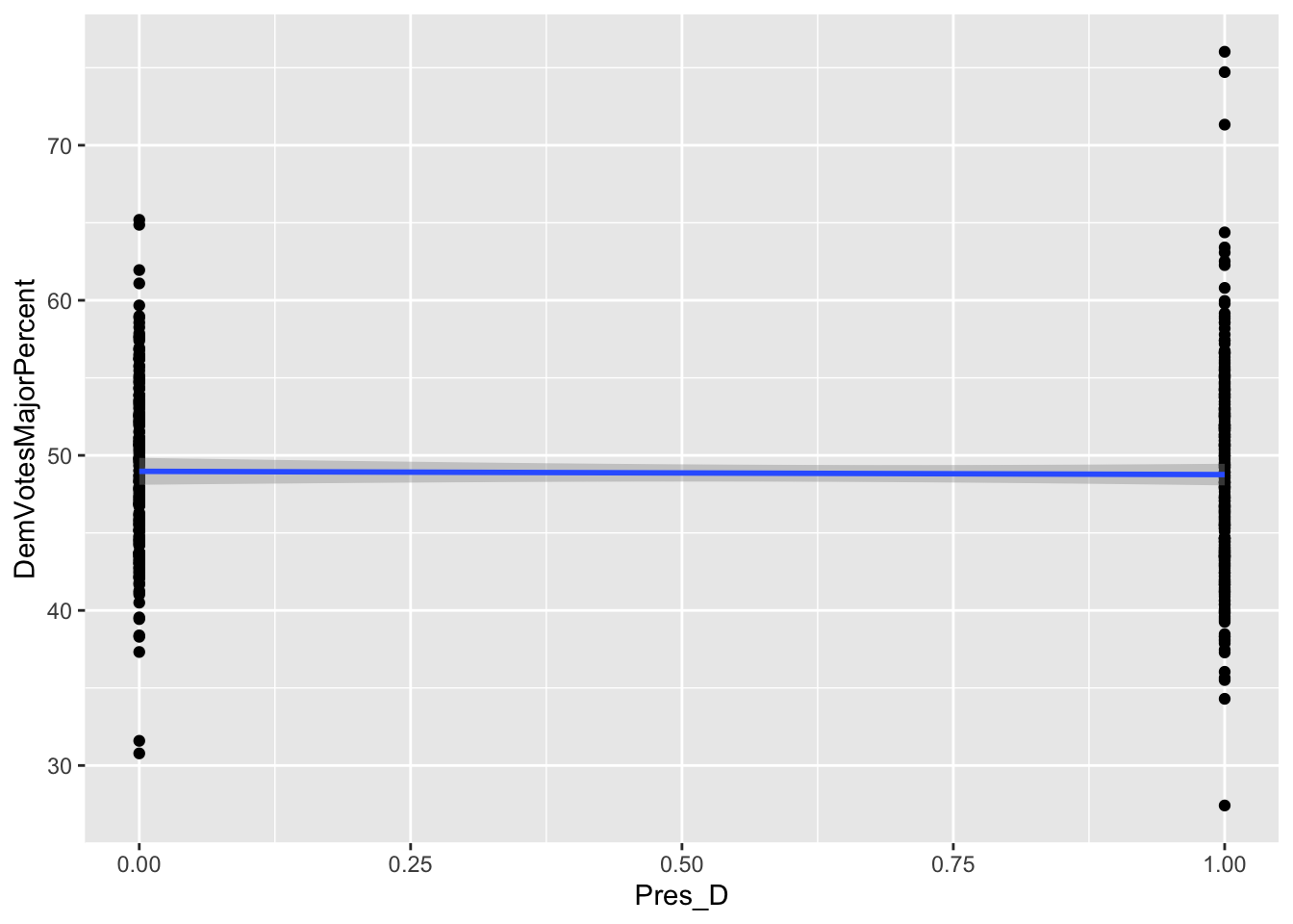
## `geom_smooth()` using formula 'y ~ x'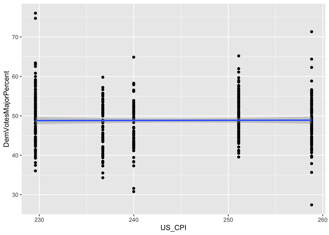
## `geom_smooth()` using formula 'y ~ x'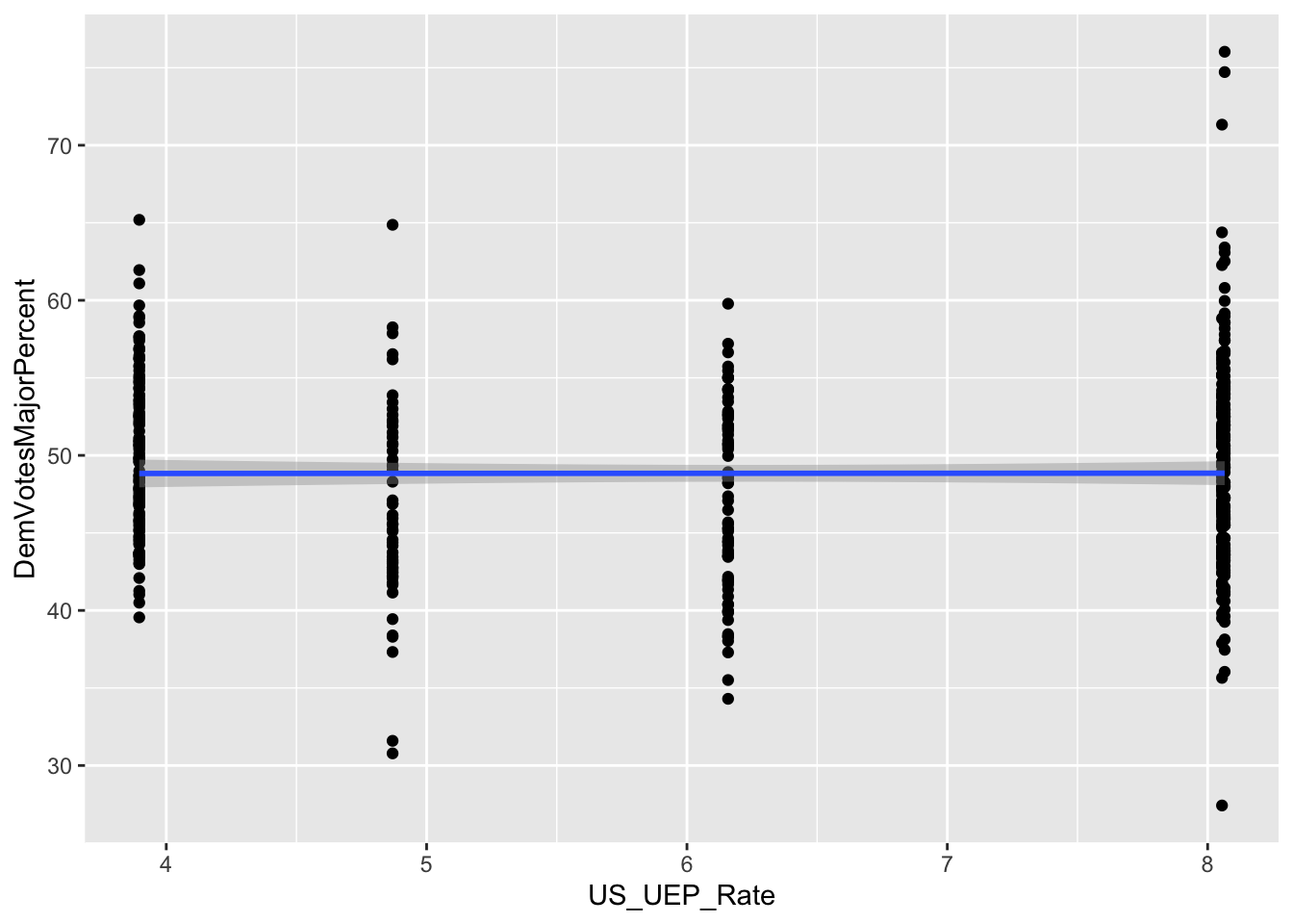
## `geom_smooth()` using formula 'y ~ x'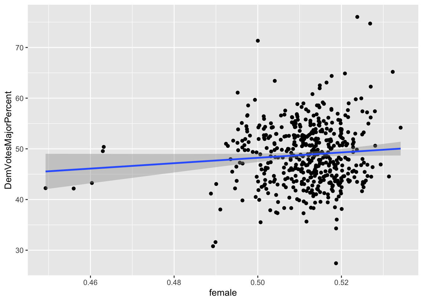
## `geom_smooth()` using formula 'y ~ x'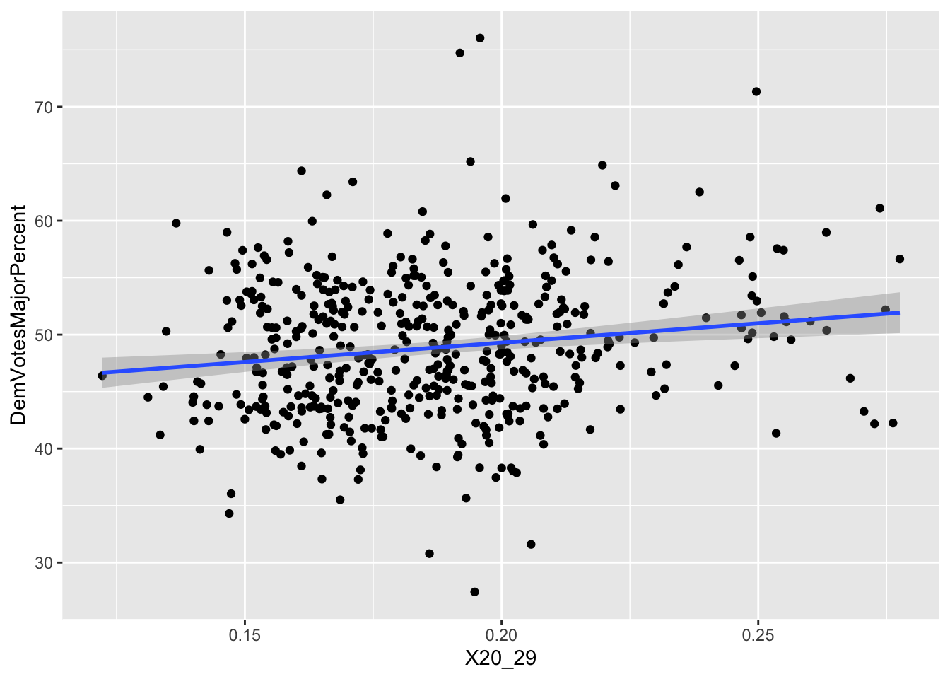
## `geom_smooth()` using formula 'y ~ x'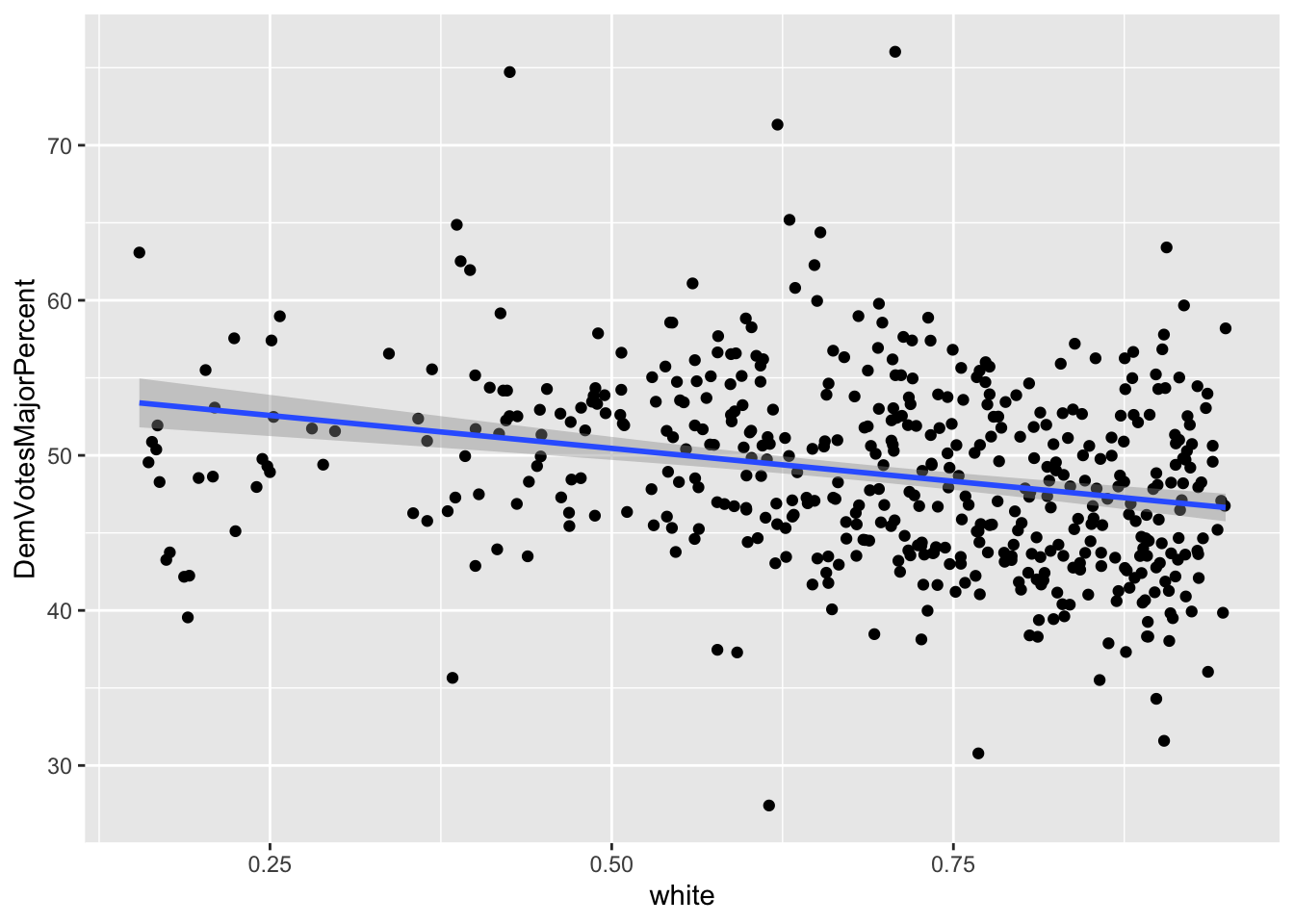 Graphed Relationship between the Dependent and Independent Variables:
A set of eight graphs shows the correlations between the dependent variable (Democrat Vote Share of the total votes to two parties) and each of the independent variables included in the prediction model (X1 through X8). The variables with dummy values, X1 (Close_E_D), X2 (LLS_D), and X3 (Pres_D), for Political Environment have only two values (0 and 1) on the horizontal axis showing the two choices of the dummy variables. The independent variables that vary only by election years are the Macroeconomic Performance variables, X4, (US_CPI), and X5 (US_UEP_Rate). These variables have the same values for all the observations in the same year. Finally, the Demographic Characteristics variables, X6 (female), X7 (X20_29), and X8 (white), vary by election years and congressional districts.
For all the correlations, the slope of the best fitted line (in blue color) is proportional to the coefficient of the multivariate regression model. Also, negative slope of a correlation indicates the direction of the marginal effect which is proportional to the slope when significant.